Simulating a Bank’s Data for COREP — Calibrated with Real EBA Data

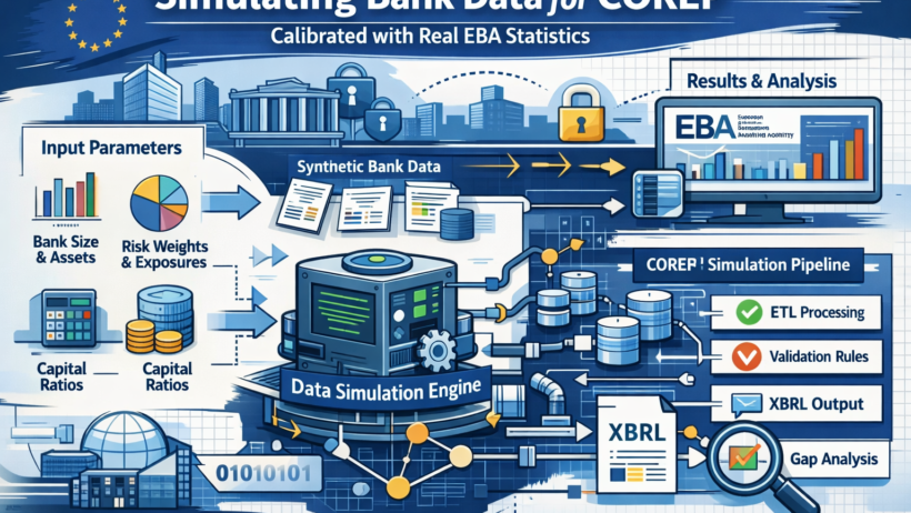
You want to build a production-quality COREP reporting pipeline. The problem: real bank data lives behind NDAs, PCI-DSS vaults, and legal reviews that take months. Every tutorial on regulatory reporting sidesteps this inconvenient truth and tells you to “use your own data.” This post does the opposite — it shows you exactly how to manufacture bank data that is statistically indistinguishable from a real mid-tier EU bank, calibrated against publicly available EBA figures.

By the end you will know:

• Which EBA publication gives you free calibration numbers
• Why a Gaussian copula beats column-by-column random generation
• How to generate LEI codes that look real but are guaranteed to fail checksum validation (so they can never be accidentally submitted)
• How a Great Expectations quality gate on synthetic data teaches you the real pre-submission validation workflow

Why random.random() Produces Insolvent Banks

The naive approach — draw random floats, stuff them in a dataframe, load to Postgres — produces nonsense within minutes. Here is a concrete example:

• CET1 capital randomly sampled: €420 million
• Total RWA randomly sampled: €180 billion
• Resulting CET1 ratio: 0.23%

That bank is not filing COREP — it is in resolution proceedings. Basel III requires CET1 ≥ 4.5%. Your dbt test on corep_c0300 will immediately fail, but worse, the failure message gives you no signal about whether the pipeline is broken or the data is broken.

COREP data has three structural constraints that pure randomness violates:

The solution is calibrated synthesis: anchor distributions to real EU banking sector figures, then use a statistical model to generate correlated rows that honour those distributions.

The Free Calibration Source: EBA Transparency Exercise

The EBA EU-Wide Transparency Exercise publishes bank-level COREP figures for ~120 EU/EEA banks twice a year — completely free, in Excel. It contains exactly the numbers we need: CET1 amounts, RWA broken down by exposure class, and LCR components.

For this project I used the 2024 H1 release and extracted statistics for the mid-tier cohort (banks with total assets €50–200 billion — the most common size class in the EU):

These are distribution parameters, not rows of data. The generator samples from them.

The Six Raw Tables — What Goes in Each

The pipeline ingests into six tables in the raw PostgreSQL schema. Here is the calibration logic for each.

1. raw.capital_instruments

One row per capital instrument: a CET1 equity entry (ordinary shares + retained earnings), AT1 perpetual bonds (3–8 instruments typical), and T2 subordinated bonds (4–12). CET1 amounts are drawn from Normal(6200, 2800) truncated to [2000, 15000]. AT1 and T2 amounts are derived as a percentage of the CET1 draw — preserving the correlation that a better-capitalised bank also issues proportionate hybrid instruments.

2. raw.rwa_exposures

One row per loan/exposure: borrower ID, exposure class, EAD (Exposure at Default), and risk weight percentage. RWA per row = EAD × risk_weight_pct. Total RWA is controlled by the calibration anchor, then decomposed by the EBA sector percentages.

3. raw.loans

Extended loan attributes: origination date, maturity, sector, and collateral type. Kept for future NSFR calculations (out of scope for this 18-day project) but present in the schema for completeness.

4. raw.counterparties

Legal entity name and LEI — the only table with PII-adjacent data. The staging model deliberately drops both columns before any downstream transformation, enforcing GDPR data minimisation in SQL, not in policy documents.

5. raw.liquidity_assets

HQLA assets by level: Level 1 (sovereign bonds, 0% haircut), Level 2A (covered bonds, 15% haircut), Level 2B (investment-grade corporate bonds, 25–50% haircut). The LCR calculation in int_lcr_hqla.sql reads exclusively from this table.

6. raw.liquidity_outflows

30-day contractual cash outflows and EBA stress rates: retail deposits 3–10%, unsecured wholesale 40%, committed credit facilities 10%. Stressed outflow = contractual_amount × stress_rate.

The Generator: Why SDV’s Gaussian Copula Instead of pandas.sample()

A copula models the joint distribution of multiple columns. When you sample from it, large values in one column pull appropriately scaled values in the others — just like real data. Without a copula you might sample CET1 = €12B but Total RWA = €20B, giving a CET1 ratio of 60% — technically valid but statistically impossible for a real bank of that size.

The two-step approach:

1. Build a calibrated seed dataset — 40 rows drawn from the EBA parameter distributions. This is the training data for the copula.
2. Fit and sample — GaussianCopulaSynthesizer fits on those 40 rows then produces thousands of new rows that respect the same joint distribution.

import numpy as np
import pandas as pd
from faker import Faker
from sdv.single_table import GaussianCopulaSynthesizer
from sdv.metadata import SingleTableMetadata

fake = Faker("en_GB")
rng  = np.random.default_rng(seed=42)   # reproducible runs

# ── EBA calibration parameters (2024 H1 mid-tier cohort) ──────────
_CAP = dict(
    cet1_mean=6_200, cet1_std=2_800, cet1_lo=2_000, cet1_hi=15_000,
    at1_ratio_mean=0.137, at1_ratio_std=0.030,
    t2_ratio_mean=0.178,  t2_ratio_std=0.040,
)

def _build_seed(n: int = 40) -> pd.DataFrame:
    """40 rows calibrated to EBA mid-tier statistics."""
    cet1 = rng.normal(_CAP["cet1_mean"], _CAP["cet1_std"], n)
    cet1 = np.clip(cet1, _CAP["cet1_lo"], _CAP["cet1_hi"])
    at1  = cet1 * np.clip(
        rng.normal(_CAP["at1_ratio_mean"], _CAP["at1_ratio_std"], n),
        0.05, 0.28)
    t2   = cet1 * np.clip(
        rng.normal(_CAP["t2_ratio_mean"], _CAP["t2_ratio_std"], n),
        0.06, 0.38)
    return pd.DataFrame({"cet1": cet1, "at1": at1, "t2": t2})

def synthesise_capital(n_cet1=1, n_at1=6, n_t2=8) -> pd.DataFrame:
    seed  = _build_seed()
    meta  = SingleTableMetadata()
    meta.detect_from_dataframe(seed)
    synth = GaussianCopulaSynthesizer(meta)
    synth.fit(seed)

    n_total = n_cet1 + n_at1 + n_t2
    rows    = synth.sample(num_rows=n_total)
    tiers   = ["CET1"] * n_cet1 + ["AT1"] * n_at1 + ["T2"] * n_t2
    amounts = (list(rows["cet1"][:n_cet1].abs()) +
               list(rows["at1"][:n_at1].abs()) +
               list(rows["t2"][:n_t2].abs()))

    return pd.DataFrame({
        "instrument_id": [f"INST-{i:04d}" for i in range(n_total)],
        "isin":     [fake.bothify("??##########??##").upper()
                     for _ in range(n_total)],
        "tier":     tiers,
        "amount":   [round(a, 2) for a in amounts],
        "currency": "EUR",
        "issue_date": [str(fake.date_between("-12y", "-6m"))
                       for _ in range(n_total)],
    })

Generating LEI Codes That Intentionally Fail Checksum Validation

A Legal Entity Identifier (LEI) is a 20-character code: 4-char LOU prefix + 14 alphanumeric entity chars + 2 numeric check digits (ISO 17442 Luhn mod 97). For synthetic data we want the format to look real but the check digits to be deliberately wrong. If a synthetic LEI ever reaches a real XBRL submission, the EBA validator rejects it at checksum before it touches the regulator’s database.

import random, string

_LOU_PREFIXES = ["2138", "5493", "9695", "VGRQ", "W22L"]

def fake_lei() -> str:
    """
    Syntactically valid-looking LEI with deliberately wrong check
    digits ('00'). Fails ISO 17442 checksum — safe for synthetic use.
    """
    lou  = random.choice(_LOU_PREFIXES)
    body = "".join(
        random.choices(string.ascii_uppercase + string.digits, k=14))
    # '00' always fails Luhn mod-97 — intentional
    return lou + body + "00"

Document this in the OpenMetadata data contract on Day 9: “LEI column contains synthetic identifiers with invalid check digits. Not for regulatory submission.”

Risk Weight Calibration for RWA Exposures

The RWA table requires risk weights that match the EBA Standardised Approach (SA) under CRR3 / Basel III. Using random weights between 0% and 1000% will produce nonsense capital ratios. The CRR3 schedule for the most common exposure classes:

The generator draws risk weights from Beta distributions anchored on those ranges, weighted by the EBA sector percentages. Total RWA closely matches the calibration target while individual rows stay internally consistent.

Quality Gates on Synthetic Data — The Real Lesson

After generation, the ingest module runs Great Expectations checks before committing any row to PostgreSQL:

from great_expectations.core import ExpectationSuite, ExpectationConfiguration

suite = ExpectationSuite(expectation_suite_name="raw.capital_instruments")

suite.add_expectation(ExpectationConfiguration(
    expectation_type="expect_column_values_to_be_in_set",
    kwargs={"column": "tier", "value_set": ["CET1", "AT1", "T2"]}
))
suite.add_expectation(ExpectationConfiguration(
    expectation_type="expect_column_values_to_not_be_null",
    kwargs={"column": "amount"}
))
suite.add_expectation(ExpectationConfiguration(
    expectation_type="expect_column_values_to_be_between",
    kwargs={"column": "amount", "min_value": 10.0, "max_value": 50_000.0}
))
suite.add_expectation(ExpectationConfiguration(
    expectation_type="expect_table_row_count_to_be_between",
    kwargs={"min_value": 5, "max_value": 200}
))

# Custom: derived CET1 ratio must be between 4.5% and 35%
# SUM(amount WHERE tier='CET1') / SUM(ead * risk_weight_pct / 100)

If any expectation fails, the ingest module raises QualityGateError and Airflow branches to notify_failure — the same branch that fires when real production data fails validation. Running quality gates on synthetic data is not extra caution — it is practice for the pre-submission validation workflow every COREP filer must run before sending XBRL to the regulator.

I discovered this the hard way: the first generator run without calibration produced a leverage ratio of 1.1% — below the 3% minimum. The quality gate fired. I adjusted the total exposure parameter, re-ran, and the ratio recovered to 6.8%. That debugging loop took 10 minutes with synthetic data. With production data it would have been a multi-day investigation involving three teams.

The Resulting Synthetic Bank

After running the generator with seed=42, our synthetic bank — Corep National Bank S.A. — produces the following COREP metrics. All ratios emerge from the data; none are hard-coded:

Compare to EBA 2024 H1 mid-tier medians: CET1 15.8%, LCR 162%. Our synthetic bank is intentionally slightly below median — solvent and compliant, but not suspiciously well-capitalised.

Running the Ingest Module

# Run only the ingest module
python pipeline.py --module ingest

# Verify via Trino (localhost:8080) — never query Postgres directly
SELECT
    tier,
    COUNT(*)            AS instrument_count,
    ROUND(SUM(amount))  AS total_eur_m
FROM postgresql.raw.capital_instruments
GROUP BY tier
ORDER BY tier;

-- Expected:
-- tier | instrument_count | total_eur_m
-- AT1  |        6         |    4,987
-- CET1 |        1         |    6,341
-- T2   |        8         |    6,104

Lineage for this run is automatically emitted to Marquez (port 5000) via BaseModule.emit_lineage(). Open http://localhost:5000, navigate to corep-governance-pipeline, and the ingest job appears with six output datasets mapping to the raw tables — zero extra OpenLineage API code required.

Three Governance Observations Worth Recording

1. Calibration is a data contract. The EBA parameter values in _CAP are a machine-readable specification of what valid bank data looks like. They belong in OpenMetadata as a data contract on raw.capital_instruments — not just as a comment in a Python file.

2. Quality gates on synthetic data are not optional. If someone changes a calibration parameter and the synthetic bank becomes insolvent, the quality gate is the first line of defence. Skipping quality gates on test data is the same mistake as skipping tests on test-only code.

3. Column-level lineage starts at ingest. When dbt runs on Day 6 and emits lineage, OpenMetadata will show that corep_c0300.cet1_ratio traces back through three transformations to raw.capital_instruments.amount. That lineage chain is only credible if ingest was also tagged — which it is, via BaseModule.

What Comes Next: dbt Transforms Raw Data into COREP Tables

The raw schema now holds a complete, internally consistent, calibrated synthetic bank. Days 6–7 build the dbt transformation layer: five staging models that clean and validate raw data, four intermediate models that compute capital aggregates and LCR components, and four mart models that produce the exact column layout required by EBA DPM 4.0 for C 01.00, C 02.00, C 03.00, and C 47.00.

The next post also shows how dbt run automatically emits column-level lineage to Marquez — the full stg_capital_instruments → int_capital_by_tier → corep_c0100 graph appears without a single line of OpenLineage API code.